
完整推导逻辑链
- 首先,DDPM总体优化目标是让模型产生的图片分布和真实图片分布尽量相似,也就是
。 - 对KL散度做初步拆解,将优化目标
转变为 ,同时也等价于让连乘项中的每一项 最大 - 继续对
做拆解,以优化DDPM其中一个time_step为例,将优化目标转向最大化下界(ELBO) - 依照马尔可夫性质,从1个time_step推至所有的time_steps,将(3)中的优化目标改写为
- 对(4)继续做拆解,将优化目标变为
- 先来看(5)中的
一项,注意到这和diffusion的过程密切相关。在diffusion的过程中,通过重参数的方法进行加噪,再经过一顿爆肝推导,得出 ,易看出该分布中方差是只和我们设置的超参数相关的常量。 - 再来看(5)中的
一项,下标说明了该项和模型相关。为了让p和q的分布接近,我们需要让p去学习q的均值和方差。由于方差是一个常量,在DDPM中,假设它是固定的,不再单独去学习它(后续的扩散模型,例如GLIDE则同时对方差也做了预测)。因此现在只需要学习q的均值。经过一顿变式,可以把q的均值改写成
。因此,这里只要让模型去预测噪声 ,使得 ,就能达到(1)中的目的
整体代码实现
DDPM原作代码地址https://github.com/hojonathanho/diffusion,采用tensorflow实现
本文采用代码地址https://github.com/labmlai/annotated_deep_learning_paper_implementations/tree/master/labml_nn/diffusion/ddpm,采用pytorch实现
Denoise Model
class DenoiseDiffusion:
    """
    Denoise Diffusion
    """

    def __init__(self, eps_model: nn.Module, n_steps: int, device: torch.device):
        """
        构造扩散模型核心组件并预计算调度超参数

        Params:
            eps_model: UNet去噪模型
            n_steps:训练总步数T
            device:训练所用硬件

        """
        super().__init__()
        # 定义UNet架构模型
        self.eps_model = eps_model
        # 人为设置超参数beta,满足beta随着t的增大而增大,同时将beta搬运到训练硬件上
        # torch.linspace(start, end, steps):创建从start开始,end结束,以steps为步长的张量
        self.beta = torch.linspace(0.0001, 0.02, n_steps).to(device)
        # 根据beta计算alpha
        self.alpha = 1. - self.beta
        # 根据alpha计算alpha_bar
        # torch.cumprod(input, dim):对输入张量input进行dim维累积乘积运算
        self.alpha_bar = torch.cumprod(self.alpha, dim=0)
        # 定义训练总步长
        self.n_steps = n_steps
        # sampling中的sigma_t
        self.sigma2 = self.beta

    def q_xt_x0(self, x0: torch.Tensor, t: torch.Tensor) -> Tuple[torch.Tensor, torch.Tensor]:
        """
        前向扩散 q(x_t | x_0) 的高斯分布参数计算。根据闭式公式 xt = sqrt(ᾱ_t) * x0 + sqrt(1 - ᾱ_t) *  ε,返回该分布的均值与方差(均值 = sqrt(ᾱ_t) * x0,方差 = 1 - ᾱ_t)

        Diffusion Process的中间步骤,根据x0和t,推导出xt所服从的高斯分布的mean和var
        Params:
            x0:来自训练数据的干净的图片
            t:某一步time_step
        Return:
            mean: xt所服从的高斯分布的均值
            var:xt所服从的高斯分布的方差

        """

        # ----------------------------------------------------------------
        # gather:人为定义的函数,从一连串超参中取出当前t对应的超参alpha_bar
        # 由于xt = sqrt(alpha_bar_t) * x0 + sqrt(1-alpha_bar_t) * epsilon
        # 其中epsilon~N(0, I)
        # 因此根据高斯分布性质,xt~N(sqrt(alpha_bar_t) * x0, 1-alpha_bar_t)
        # 即为本步中我们要求的mean和var
        # ----------------------------------------------------------------
        mean = gather(self.alpha_bar, t) ** 0.5 * x0
        var = 1 - gather(self.alpha_bar, t)

        return mean, var

    def q_sample(self, x0: torch.Tensor, t: torch.Tensor, eps: Optional[torch.Tensor] = None):
        """
        执行前向扩散采样:从 q(x_t | x_0) 抽样得到 x_t。利用闭式公式与随机噪声 ε ~ N(0, I),生成指定时间步 t 的带噪样本 x_t

        Diffusion Process,根据xt所服从的高斯分布的mean和var,求出xt
        Params:
            x0:来自训练数据的干净的图片
            t:某一步time_step
        Return:
            xt: 第t时刻加完噪声的图片

        """

        # ----------------------------------------------------------------
        # xt = sqrt(alpha_bar_t) * x0 + sqrt(1-alpha_bar_t) * epsilon
        #    = mean + sqrt(var) * epsilon
        # 其中,epsilon~N(0, I)
        # ----------------------------------------------------------------
        if eps is None:
            # torch.randn_like(x):创建一个与x大小相同的新张量
            eps = torch.randn_like(x0)

        mean, var = self.q_xt_x0(x0, t)
        return mean + (var ** 0.5) * eps

    def p_sample(self, xt: torch.Tensor, t: torch.Tensor):
        """
        反向采样一步:根据当前模型预测,从 x_t 还原到 x_{t-1}。用 ε_θ(x_t, t) 近似真实噪声,依据 DDPM 的后验均值闭式公式,计算 p_θ(x_{t-1} | x_t) 的均值与方差并进行采样

        Sampling, 当模型训练好之后,根据x_t和t,推出x_{t-1}
        Params:
            x_t:t时刻的图片
            t:某一步time_step
        Return:
            x_{t-1}: 第t-1时刻的图片

        """

        # eps_model: 训练好的UNet去噪模型
        # eps_theta: 用训练好的UNet去噪模型,预测第t步的噪声
        eps_theta = self.eps_model(xt, t)

        # 根据Sampling提供的公式,推导出x_{t-1}
        alpha_bar = gather(self.alpha_bar, t)
        alpha = gather(self.alpha, t)
        eps_coef = (1 - alpha) / (1 - alpha_bar) ** .5
        mean = 1 / (alpha ** 0.5) * (xt - eps_coef * eps_theta)
        var = gather(self.sigma2, t)
        # torch.randn(size):生成服从标准正态分布的随机张量,size定义输出张量的形状
        eps = torch.randn(xt.shape, device=xt.device)

        return mean + (var ** .5) * eps

    def loss(self, x0: torch.Tensor, noise: Optional[torch.Tensor] = None):
        """
        单步损失计算:随机采样时间步 t,比较真实噪声与模型预测噪声的 MSE

        1. 随机抽取一个time_step t
        2. 执行diffusion process(q_sample),随机生成噪声epsilon~N(0, I),
           然后根据x0, t和epsilon计算xt
        3. 使用UNet去噪模型(p_sample),根据xt和t得到预测噪声epsilon_theta
        4. 计算mse_loss(epsilon, epsilon_theta)

        【MSE只是众多可选loss设计中的一种,也可以自行设计loss函数】

        Params:
            x0:来自训练数据的干净的图片
            noise: diffusion process中随机抽样的噪声epsilon~N(0, I)
        Return:
            loss: 真实噪声和预测噪声之间的loss

        """

        batch_size = x0.shape[0]
        # 随机抽样t
        # torch.randint(low, high, size):生成随机整数张量,范围[low,high),size定义张量形状
        t = torch.randint(0, self.n_steps, (batch_size,), device=x0.device, dtype=torch.long)

        # 如果为传入噪声,则从N(0, I)中抽样噪声
        if noise is None:
            noise = torch.randn_like(x0)

        # 执行Diffusion process,计算xt
        xt = self.q_sample(x0, t, eps=noise)
        # 执行Denoise Process,得到预测的噪声epsilon_theta
        eps_theta = self.eps_model(xt, t)

        # 返回真实噪声和预测噪声之间的mse loss
        return F.mse_loss(noise, eps_theta)
定义好DenoiseModel后,我们就可以进一步定义train函数来训练模型了,这里我们只截取代码中的核心部分,总体来说,每个epoch的训练分成两个部分:
train(): 在这一部分中,我们创建模型(DenoiseModel),遍历所有的batch,计算loss并做梯度更新。sample():每个epoch训练完毕后,我们根据上图sample部分中的公式,利用当前的模型,将一张高斯噪声()逐步还原回 , 将用于评估当前模型的效果(例如计算FID之类)
def train(self):
   """
   单epoch训练DDPM:遍历数据批次,计算扩散损失并进行梯度更新
   """

   # 遍历每一个batch(monit是自定义类,详情参见github完整代码)
   for data in monit.iterate('Train', self.data_loader):
       # step数+1(tracker是自定义类,详情参见github完整代码)
       tracker.add_global_step()
       # 将这个batch的数据移动到GPU上
       data = data.to(self.device)

       # 每个batch开始时,梯度清0
       self.optimizer.zero_grad()
       # self.diffusion即为DenoiseModel实例,执行forward,计算loss
       loss = self.diffusion.loss(data)
       # 计算梯度
       loss.backward()
       # 更新
       self.optimizer.step()
       # 保存loss,用于后续可视化之类的操作
       tracker.save('loss', loss)

def sample(self):
    """
    生成评估样本:从高斯噪声出发,按时间步迭代反向采样至 x0

    利用当前模型,将一张随机高斯噪声(xt)逐步还原回x0,
    x0将用于评估模型效果(例如FID分数)

    """
    with torch.no_grad():
        # 随机抽取n_samples张纯高斯噪声
        x = torch.randn([self.n_samples, self.image_channels, self.image_size, self.image_size],
                            device=self.device)

        # 对每一张噪声,按照sample公式,还原回x0
        for t_ in monit.iterate('Sample', self.n_steps):
            t = self.n_steps - t_ - 1
            x = self.diffusion.p_sample(x, x.new_full((self.n_samples,), t, dtype=torch.long))

        # 保存x0
        tracker.save('sample', x)

def run(self):
    """
    train主函数:逐 epoch 调用训练与采样,并保存检查点
    """
    # 遍历每一个epoch
    for _ in monit.loop(self.epochs):
        # 训练模型
        self.train()
        # 利用当前训好的模型做sample,从xt还原x0,保存x0用于后续效果评估
        self.sample()
        # 再console上新起一行
        tracker.new_line()
        # 保存模型(experiment是自定义类,详情参见github代码)
        experiment.save_checkpoint()
Unet
主体架构
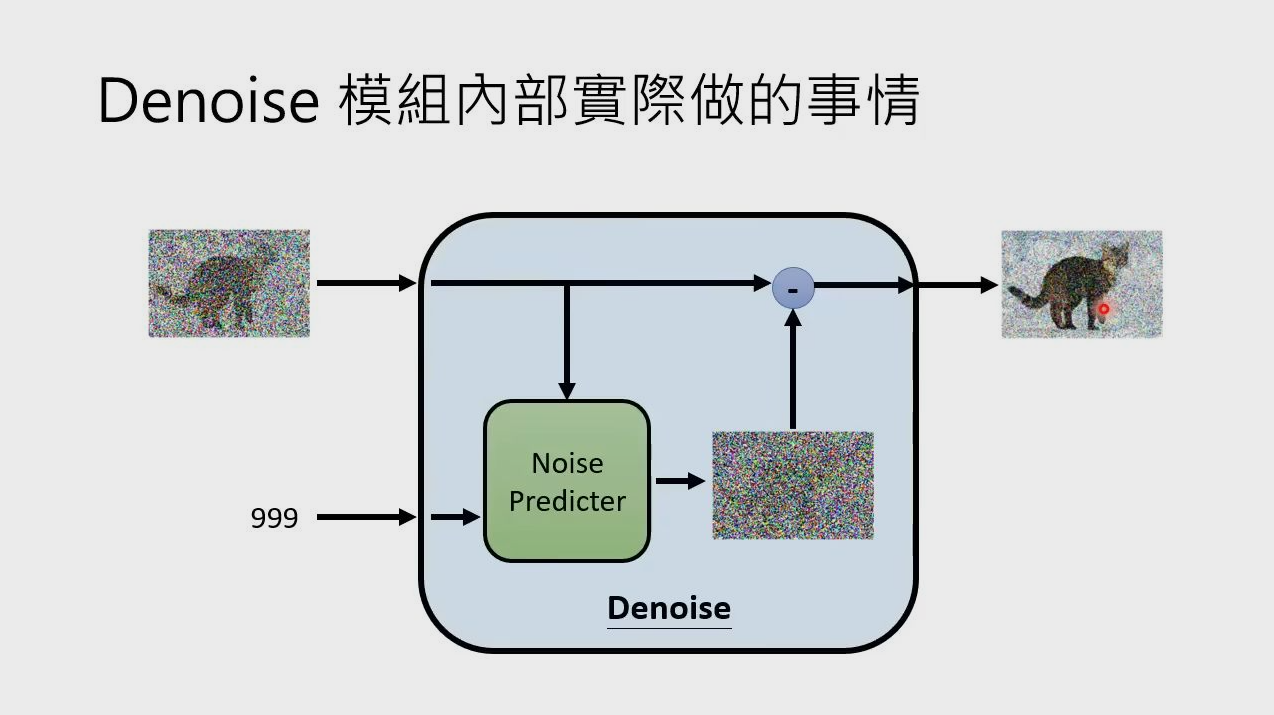
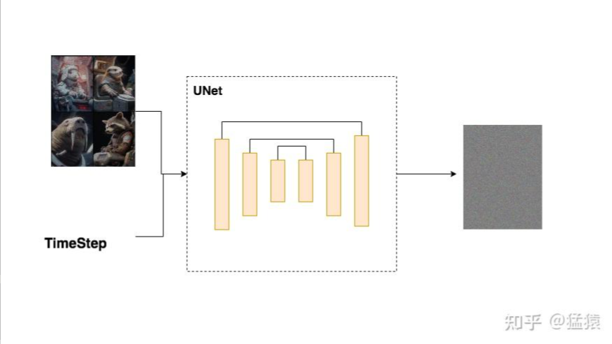
- DDPM UNet的输入是某一时刻的图片 和用于表示该时刻的t向量
- DDPM UNet的输出是对t时刻噪声的预测。
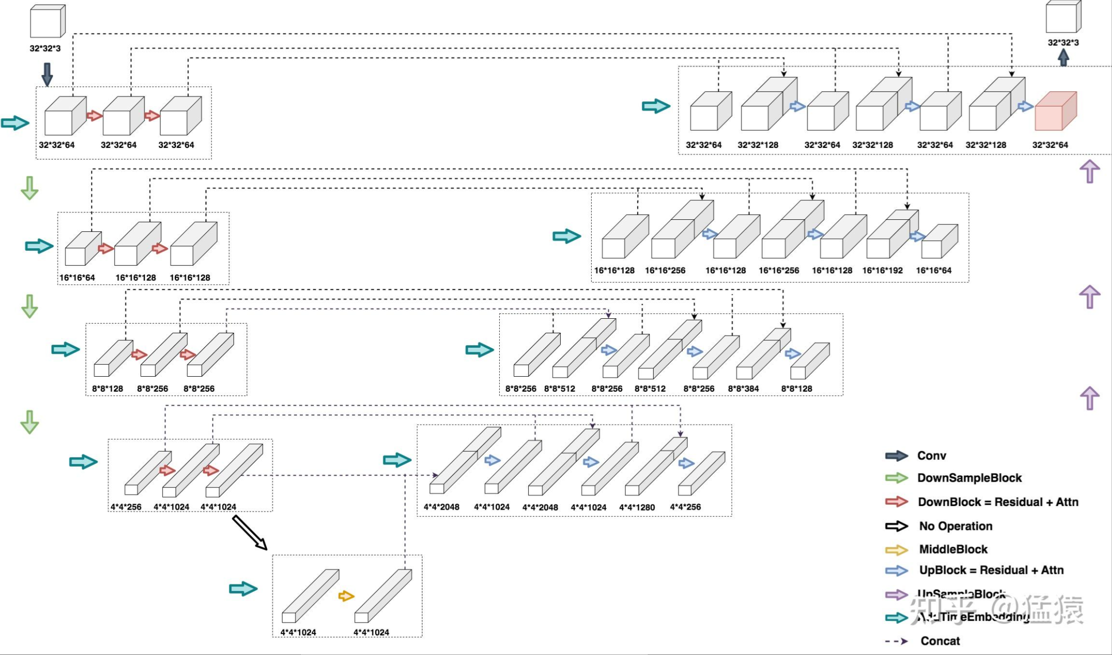
- DDPM UNet是一个典型的Encoder-Decoder结构,在Encoder中,我们压缩图片大小,逐步提取图片特征;在Decoder中,我们逐步还原图片大小。由于压缩图片可能会损失掉信息,因此在decoder做还原时,我们会拼接Encoder层对应的特征图(skip connection),尽量减少信息损失。
class UNet(Module):
    """
    DDPM UNet去噪模型主体架构
    """

    def __init__(self, image_channels: int = 3, n_channels: int = 64,
                 ch_mults: Union[Tuple[int, ...], List[int]] = (1, 2, 2, 4),
                 is_attn: Union[Tuple[bool, ...], List[int]] = (False, False, True, True),
                 n_blocks: int = 2):
        """
        时序条件 UNet 主体:编码器-中间层-解码器结构,用于预测噪声 ε_θ

        Params:
            image_channels:原始输入图片的channel数,对RGB图像来说就是3

            n_channels:    在进UNet之前,会对原始图片做一次初步卷积,该初步卷积对应的
                            out_channel数,也就是图中左上角的第一个墨绿色箭头

            ch_mults:      在Encoder下采样的每一层的out_channels倍数,
                            例如ch_mults[i] = 2,表示第i层特征图的out_channel数,
                            是第i-1层的2倍。Decoder上采样时也是同理,用的是反转后的ch_mults

            is_attn:       在Encoder下采样/Decoder上采样的每一层,是否要在CNN做特征提取后再引入attention

            n_blocks:      在Encoder下采样/Decoder下采样的每一层,需要用多少个DownBlock/UpBlock(见图),
                            Deocder层最终使用的UpBlock数=n_blocks + 1

        """
        super().__init__()

        # 在Encoder下采样/Decoder上采样的过程中,图像依次缩小/放大,
        # 每次变动都会产生一个新的图像分辨率
        # 这里指的就是不同图像分辨率的个数,也可以理解成是Encoder/Decoder的层数
        n_resolutions = len(ch_mults)

        # 对原始图片做预处理,例如图中,将32*32*3 -> 32*32*64
        self.image_proj = nn.Conv2d(image_channels, n_channels, kernel_size=(3, 3), padding=(1, 1))

        # time_embedding,TimeEmbedding是nn.Module子类,我们会在下文详细讲解它的属性和forward方法
        self.time_emb = TimeEmbedding(n_channels * 4)

        # --------------------------
        # 定义Encoder部分
        # --------------------------
        # down列表中的每个元素表示Encoder的每一层
        down = []
        # 初始化out_channel和in_channel
        out_channels = in_channels = n_channels
        # 遍历每一层
        for i in range(n_resolutions):
            # 根据设定好的规则,得到该层的out_channel
            out_channels = in_channels * ch_mults[i]
            # 根据设定好的规则,每一层有n_blocks个DownBlock
            for _ in range(n_blocks):
                down.append(DownBlock(in_channels, out_channels, n_channels * 4, is_attn[i]))
                in_channels = out_channels
            # 对Encoder来说,每一层结束后,我们都做一次下采样,但Encoder的最后一层不做下采样
            if i < n_resolutions - 1:
                down.append(Downsample(in_channels))

        # self.down即是完整的Encoder部分
        self.down = nn.ModuleList(down)

        # --------------------------
        # 定义Middle部分
        # --------------------------
        self.middle = MiddleBlock(out_channels, n_channels * 4, )

        # --------------------------
        # 定义Decoder部分
        # --------------------------

        # 和Encoder部分基本一致,可对照绘制的架构图阅读
        up = []
        in_channels = out_channels
        for i in reversed(range(n_resolutions)):
            # `n_blocks` at the same resolution
            out_channels = in_channels
            for _ in range(n_blocks):
                up.append(UpBlock(in_channels, out_channels, n_channels * 4, is_attn[i]))

            out_channels = in_channels // ch_mults[i]
            up.append(UpBlock(in_channels, out_channels, n_channels * 4, is_attn[i]))
            in_channels = out_channels

            if i > 0:
                up.append(Upsample(in_channels))

        # self.up即是完整的Decoder部分
        self.up = nn.ModuleList(up)

        # 定义group_norm, 激活函数,和最后一层的CNN(用于将Decoder最上一层的特征图还原成原始尺寸)
        self.norm = nn.GroupNorm(8, n_channels)
        self.act = Swish()
        self.final = nn.Conv2d(in_channels, image_channels, kernel_size=(3, 3), padding=(1, 1))

    def forward(self, x: torch.Tensor, t: torch.Tensor):
        """
        前向计算:预测给定 `x_t` 在时间步 `t` 的噪声 ε_θ

        Params:
            x: 输入数据xt,尺寸大小为(batch_size, in_channels, height, width)
            t: 输入数据t,尺寸大小为(batch_size)

        """

        # 取得time_embedding
        t = self.time_emb(t)

        # 对原始图片做初步CNN处理
        x = self.image_proj(x)

        # -----------------------
        # Encoder
        # -----------------------
        h = [x]
        # First half of U-Net
        for m in self.down:
            x = m(x, t)
            h.append(x)

        # -----------------------
        # Middle
        # -----------------------
        x = self.middle(x, t)

        # -----------------------
        # Decoder
        # -----------------------
        for m in self.up:
            if isinstance(m, Upsample):
                x = m(x, t)
            else:
                s = h.pop()
                # skip_connection
                x = torch.cat((x, s), dim=1)
                x = m(x, t)

        return self.final(self.act(self.norm(x)))
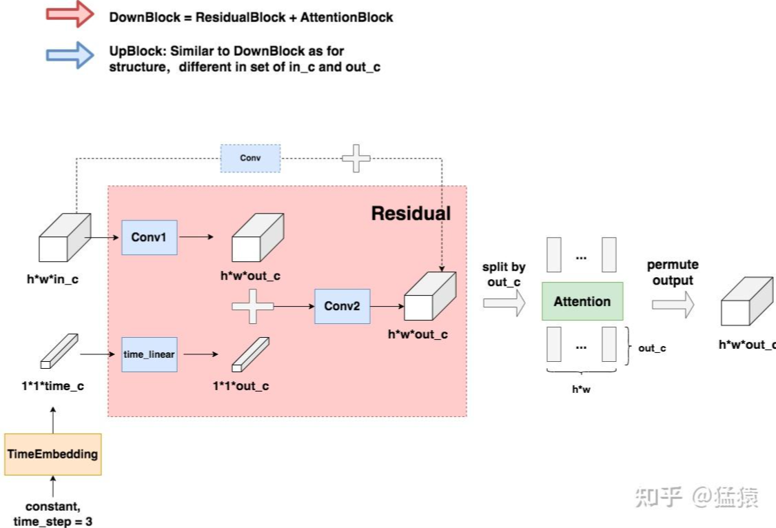
DownBlock 和 UpBlock
DownBlock和UpBlock的内部架构非常相似,都是Redisual + Attention,其中Attention部分不是必须的,是可选的。这里只摘取DownBlock部分的代码进行讲解
class ResidualBlock(Module):
    """
    每一个Residual block都有两层CNN做特征提取
    """

    def __init__(self, in_channels: int, out_channels: int, time_channels: int,
                 n_groups: int = 32, dropout: float = 0.1):
        """
        带时间调制的二维卷积残差块(GN + Swish + Conv),两层卷积并支持通道映射

        Params:
            in_channels:  输入图片的channel数量
            out_channels: 经过residual block后输出特征图的channel数量
            time_channels:time_embedding的向量维度,例如t原来是个整型,值为1,表示时刻1,
                           现在要将其变成维度为(1, time_channels)的向量
            n_groups:     Group Norm中的超参
            dropout:      dropout rate
        """
        super().__init__()

        # 第一层卷积 = Group Norm + CNN
        self.norm1 = nn.GroupNorm(n_groups, in_channels)
        self.act1 = Swish()
        self.conv1 = nn.Conv2d(in_channels, out_channels, kernel_size=(3, 3), padding=(1, 1))

        # 第二层卷积 = Group Norm + CNN
        self.norm2 = nn.GroupNorm(n_groups, out_channels)
        self.act2 = Swish()
        self.conv2 = nn.Conv2d(out_channels, out_channels, kernel_size=(3, 3), padding=(1, 1))

        # 当in_c = out_c时,残差连接直接将输入输出相加;
        # 当in_c != out_c时,对输入数据做一次卷积,将其通道数变成和out_c一致,再和输出相加
        if in_channels != out_channels:
            self.shortcut = nn.Conv2d(in_channels, out_channels, kernel_size=(1, 1))
        else:
            self.shortcut = nn.Identity()

        # t向量的维度time_channels可能不等于out_c,所以我们要对起做一次线性转换
        self.time_emb = nn.Linear(time_channels, out_channels)
        self.time_act = Swish()

        self.dropout = nn.Dropout(dropout)

    def forward(self, x: torch.Tensor, t: torch.Tensor):
        """
        前向计算:应用两层卷积与时间调制并进行残差加和

        Params:
            x: 输入数据xt,尺寸大小为(batch_size, in_channels, height, width)
            t: 输入数据t,尺寸大小为(batch_size, time_c)

        """
        # 1.输入数据先过一层卷积
        h = self.conv1(self.act1(self.norm1(x)))
        # 2. 对time_embedding向量,通过线性层使time_c变为out_c,再和输入数据的特征图相加
        h += self.time_emb(self.time_act(t))[:, :, None, None]
        # 3、过第二层卷积
        h = self.conv2(self.dropout(self.act2(self.norm2(h))))

        # 4、返回残差连接后的结果
        return h + self.shortcut(x)


class AttentionBlock(Module):
    """
    Attention模块
    和Transformer中的multi-head attention原理及实现方式一致
    """

    def __init__(self, n_channels: int, n_heads: int = 1, d_k: int = None, n_groups: int = 32):
        """
        二维特征上的多头自注意力块(通道视为 token 维度或经重排)

        Params:
            n_channels:等待做attention操作的特征图的channel数
            n_heads:   attention头数
            d_k:       每一个attention头处理的向量维度
            n_groups:  Group Norm超参数
        """
        super().__init__()

        # 一般而言,d_k = n_channels // n_heads,需保证n_channels能被n_heads整除
        if d_k is None:
            d_k = n_channels
        # 定义Group Norm
        self.norm = nn.GroupNorm(n_groups, n_channels)
        # Multi-head attention层: 定义输入token分别和q,k,v矩阵相乘后的结果
        self.projection = nn.Linear(n_channels, n_heads * d_k * 3)
        # MLP层
        self.output = nn.Linear(n_heads * d_k, n_channels)

        self.scale = d_k ** -0.5
        self.n_heads = n_heads
        self.d_k = d_k

    def forward(self, x: torch.Tensor, t: Optional[torch.Tensor] = None):
        """
        前向计算:对特征图应用多头自注意力并返回同形输出

        Params:
            x: 输入数据xt,尺寸大小为(batch_size, in_channels, height, width)
            t: 输入数据t,尺寸大小为(batch_size, time_c)

        """
        # t并没有用到,但是为了和ResidualBlock定义方式一致,这里也引入了t
        _ = t
        # 获取shape
        batch_size, n_channels, height, width = x.shape
        # 将输入数据的shape改为(batch_size, height*weight, n_channels)
        # 这三个维度分别等同于transformer输入中的(batch_size, seq_length, token_embedding)
        # (参见图例)
        x = x.view(batch_size, n_channels, -1).permute(0, 2, 1)
        # 计算输入过矩阵q,k,v的结果,self.projection通过矩阵计算,一次性把这三个结果出出来
        # 也就是qkv矩阵是三个结果的拼接
        # 其shape为:(batch_size, height*weight, n_heads, 3 * d_k)
        qkv = self.projection(x).view(batch_size, -1, self.n_heads, 3 * self.d_k)
        # 将拼接结果切开,每一个结果的shape为(batch_size, height*weight, n_heads, d_k)
        q, k, v = torch.chunk(qkv, 3, dim=-1)
        # 以下是正常计算attention score的过程,不再做说明
        attn = torch.einsum('bihd,bjhd->bijh', q, k) * self.scale
        attn = attn.softmax(dim=2)
        res = torch.einsum('bijh,bjhd->bihd', attn, v)
        # 将结果reshape成(batch_size, height*weight,, n_heads * d_k)
        # 复习一下:n_heads * d_k = n_channels
        res = res.view(batch_size, -1, self.n_heads * self.d_k)
        # MLP层,输出结果shape为(batch_size, height*weight,, n_channels)
        res = self.output(res)

        # 残差连接
        res += x

        # 将输出结果从序列形式还原成图像形式,
        # shape为(batch_size, n_channels, height, width)
        res = res.permute(0, 2, 1).view(batch_size, n_channels, height, width)

        return res


class DownBlock(Module):
    """
    Down block,即Encoder中每一层的核心处理逻辑
    DownBlock = ResidualBlock + AttentionBlock
    在我们的例子中,Encoder的每一层都有2个DownBlock
    """

    def __init__(self, in_channels: int, out_channels: int, time_channels: int, has_attn: bool):
        super().__init__()
        self.res = ResidualBlock(in_channels, out_channels, time_channels)
        if has_attn:
            self.attn = AttentionBlock(out_channels)
        else:
            self.attn = nn.Identity()

    def forward(self, x: torch.Tensor, t: torch.Tensor):
        x = self.res(x, t)
        x = self.attn(x)
        return x
TimeEmbedding
- 我们定义TimeEmbedding模块,将这个整数包装成维度=time_channel的向量,这个包装方式和Transformer中函数式位置编码的包装方式一致。
- 然后,再实际应用到time_emebdding向量时,再通过一个简单的线性层,将其维度从time_channel转变为对应特征图的out_channel,使其能够和特征图相加。
class TimeEmbedding(nn.Module):
    """
    TimeEmbedding模块将把整型t,以Transformer函数式位置编码的方式,映射成向量,
    其shape为(batch_size, time_channel)
    """

    def __init__(self, n_channels: int):
        """
        Params:
            n_channels:即time_channel
        """
        super().__init__()
        self.n_channels = n_channels
        self.lin1 = nn.Linear(self.n_channels // 4, self.n_channels)
        self.act = Swish()
        self.lin2 = nn.Linear(self.n_channels, self.n_channels)

    def forward(self, t: torch.Tensor):
        """
        Params:
            t: 维度(batch_size),整型时刻t
        """
        # 以下转换方法和Transformer的位置编码一致
        half_dim = self.n_channels // 8
        emb = math.log(10_000) / (half_dim - 1)
        emb = torch.exp(torch.arange(half_dim, device=t.device) * -emb)
        emb = t[:, None] * emb[None, :]
        emb = torch.cat((emb.sin(), emb.cos()), dim=1)

        # Transform with the MLP
        emb = self.act(self.lin1(emb))
        emb = self.lin2(emb)

        # 输出维度(batch_size, time_channels)
        return emb
DownSample和UpSample
这两块分别起到“压缩特征”和“还原特征”的作用
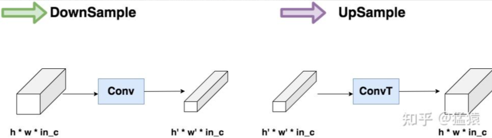
class Upsample(nn.Module):
    """
    上采样
    """

    def __init__(self, n_channels):
        super().__init__()
        self.conv = nn.ConvTranspose2d(n_channels, n_channels, (4, 4), (2, 2), (1, 1))

    def forward(self, x: torch.Tensor, t: torch.Tensor):
        _ = t
        return self.conv(x)


class Downsample(nn.Module):
    """
    下采样
    """

    def __init__(self, n_channels):
        super().__init__()
        self.conv = nn.Conv2d(n_channels, n_channels, (3, 3), (2, 2), (1, 1))

    def forward(self, x: torch.Tensor, t: torch.Tensor):
        _ = t
        return self.conv(x)
MiddleBlock
MiddleBlock = ResidualBlock + AttentionBlock + ResidualBlock组成
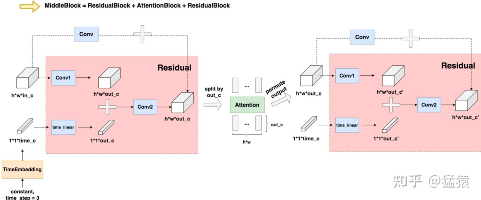
class MiddleBlock(Module):
    """
    MiddleBlock
    这是UNet结构中,连接Encoder和Decoder的最下层部分,
    MiddleBlock = ResidualBlock + AttentionBlock + ResidualBlock
    """

    def __init__(self, n_channels: int, time_channels: int):
        super().__init__()
        self.res1 = ResidualBlock(n_channels, n_channels, time_channels)
        self.attn = AttentionBlock(n_channels)
        self.res2 = ResidualBlock(n_channels, n_channels, time_channels)

    def forward(self, x: torch.Tensor, t: torch.Tensor):
        x = self.res1(x, t)
        x = self.attn(x)
        x = self.res2(x, t)
        return x
参考资料:深入浅出扩散模型(Diffusion Model)系列:基石DDPM(源码解读篇) - 猛猿的文章 - 知乎
https://zhuanlan.zhihu.com/p/655568910
Comments NOTHING